1
2
3
import pandas as pd
import seaborn as sns
import matplotlib.pyplot as plt
1
df = pd.read_csv("train.csv")
Categorical Plots
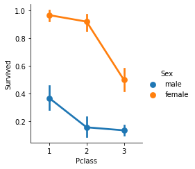
Factorplot
- seaborn.factorplot(x, y, hue, data, row, col…, aspect, size,…)
- x,y: Column 이름
- hue (option): Color encoding을 적용할 Column 이름
- data: Dataframe
- aspect(option): 실수, 가로/세로 비율
1
sns.factorplot(x="Pclass", y="Survived", hue="Sex", data=df, aspect=0.9, size=3.5)
1
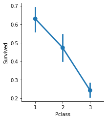
sns.factorplot(x="Pclass", y="Survived", data=df, aspect=0.9, size=3.5)
1
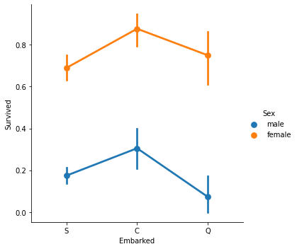
sns.factorplot(x="Embarked", y="Survived", hue="Sex", data=df)
Countplot
- 각 카테고리 값 별로 데이터가 얼마나 있는지 표시(변수의 발생 횟수)
- seaborn.countplot(x=”column_name”, data=dataframe)
1
2
3
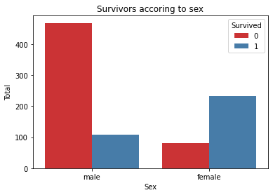
ax = sns.countplot(x="Sex", hue="Survived", palette="Set1", data=df)
ax.set(title="Survivors accoring to sex", xlabel="Sex",ylabel="Total")
plt.show()
1
2
3
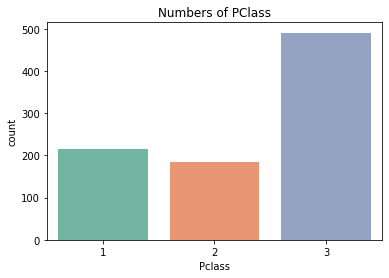
sns.countplot(x="Pclass", data=df, palette = "Set2")
plt.title("Numbers of PClass")
plt.show()
1
2
3
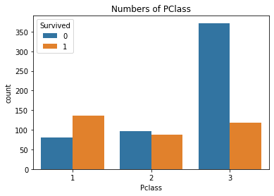
sns.countplot(x="Pclass", hue = 'Survived',data=df)
plt.title("Numbers of PClass")
plt.show()
1
df.head()
| PassengerId | Survived | Pclass | Name | Sex | Age | SibSp | Parch | Ticket | Fare | Cabin | Embarked | |
|---|---|---|---|---|---|---|---|---|---|---|---|---|
| 0 | 1 | 0 | 3 | Braund, Mr. Owen Harris | male | 22.0 | 1 | 0 | A/5 21171 | 7.2500 | NaN | S |
| 1 | 2 | 1 | 1 | Cumings, Mrs. John Bradley (Florence Briggs Th... | female | 38.0 | 1 | 0 | PC 17599 | 71.2833 | C85 | C |
| 2 | 3 | 1 | 3 | Heikkinen, Miss. Laina | female | 26.0 | 0 | 0 | STON/O2. 3101282 | 7.9250 | NaN | S |
| 3 | 4 | 1 | 1 | Futrelle, Mrs. Jacques Heath (Lily May Peel) | female | 35.0 | 1 | 0 | 113803 | 53.1000 | C123 | S |
| 4 | 5 | 0 | 3 | Allen, Mr. William Henry | male | 35.0 | 0 | 0 | 373450 | 8.0500 | NaN | S |
FacetGrid
- FacetGrid에 데이터프레임과 row, col, hue 등 전달해 객체 생성
- 객체(facet)의 map 함수에 적용할 그래프의 종류와 Column 전달
- outelier 데이터 확인 가능
1
2
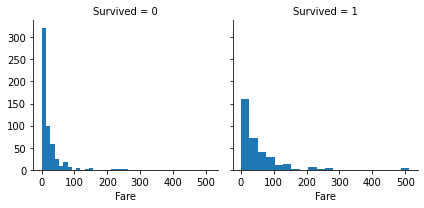
graph = sns.FacetGrid(df, col="Survived")
graph.map(plt.hist, "Fare", bins=20) # 각 서브 플롯에 적용할 그래프 종류를 map() 이용하여 그리드 객체에 전달
1
2
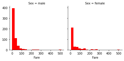
graph = sns.FacetGrid(df, col="Sex")
graph.map(plt.hist, "Fare", bins=20, color ='r')
1
2
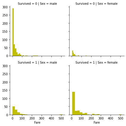
graph = sns.FacetGrid(df, col="Sex", row = "Survived")
graph = graph.map(plt.hist, "Fare", bins=20, color ='y')
1
2
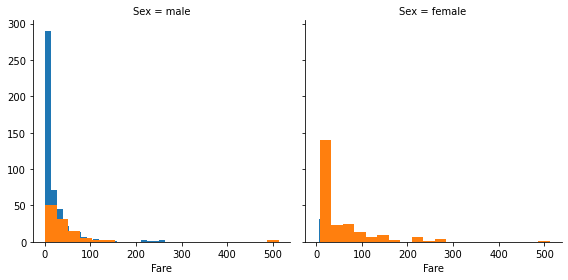
graph = sns.FacetGrid(df, col="Sex", hue = "Survived", size = 4)
graph = graph.map(plt.hist, "Fare", bins=20)
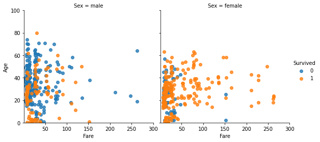
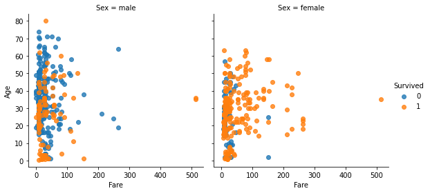
- 히스토그램 뿐만 아니라 아래와 같이 regplot을 이용하여 시각화 가능
- 색깔 별로 어떤 값을 나타내는지 legend 추가(범례 추가)
1
2
3
graph = sns.FacetGrid(df, col="Sex", hue = "Survived", size = 4)
graph = graph.map(sns.regplot, "Fare", 'Age',fit_reg=False)
graph=graph.add_legend()
- X축, Y축 범위 추가
1
2
3
4
graph = sns.FacetGrid(df, col="Sex", hue = "Survived", size = 4)
graph = graph.map(sns.regplot, "Fare", 'Age',fit_reg=False)
graph=graph.add_legend()
graph.set(xlim = (1,300), ylim=(0,100))